observing ECCO vs tidal gauges affected by Hurricane Maria - a deep dive
Table of Contents
Introduction
Sea level rise is an increase in the ocean’s surface height relative to the land in a particular location, mainly caused by expansion of warm ocean water and melting polar ice [1]. Sea surface height (SSH) can be measured in situ using tide gauges (TGs), or using satellite altimeters. Tide gauges, commonly found in water level monitoring stations, are fitted with sensors that continuously record the height of the surrounding water level [2]. On the other hand, satellite altimeters measure SSH by measuring the time it takes for microwave pulses to travel from the satellite and the lowest point of the sea surface.
Satellite altimeters assume that the pulse reflections are homogeneous. However, in coastal areas, there are various sources of inhomogeneous microwave reflections, such as land, ships, and smooth water in ports, which decrease the quality of the altimeters’ estimations of the SSH [3]. Furthermore, under the influence of extreme weather events like hurricanes, such discrepancies are further exposed due to the increased fluctuation in SSH levels. Tide gauge measurements are made with respect to a local fixed reference on land [4], therefore their measurements are more accurate, but they are susceptible to extreme weather. With this, there’s a need to consolidate SSH data measured during extreme events by tide gauges and satellite altimeters.
This article describes a Python project comparing SSH data measured from tide gauges in Puerto Rico that were affected by Hurricane Maria, and the corresponding SSH data from the same time period, sourced from satellite altimeters.
Methods
SSH data retrieval
SSH data sourcing
SSH data can be obtained from satellite altimeters and tide gauges. For the satellite source, we used ECCO, which is the abbreviation for “Estimating the Circulation and Climate of the Ocean”. We used the ECCO Version 4 Release 4 model, which covers the period from January 1992 to December 2017 [5], [6], [7]. The instructions to download the dataset follow in the referenced website. For this project, we specifically used ‘Option 2: Daily Fields on the NASA Advanced Supercomputing (NAS) ECCO Data Portal’, as shown in the website.
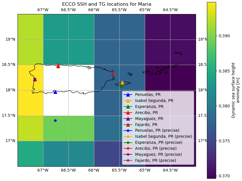
SSH data from the TGs was obtained from the University of Hawaii Sea Level Center (UHSLC) database. Since we focused on the areas affected by Hurricane Maria in Puerto Rico, we analyzed SSH data from 6 TGs, namely: Penuelas, Isabel Segunda, Esperanza, Arecibo, Mayaguez and Fajardo.
To begin with, we import the required libraries.
import matplotlib.pyplot as plt
import xarray as xr
import os
import pooch
import tempfile
from pooch import HTTPDownloader
import pandas as pd
from datetime import timedelta, datetime
import numpy as np
import matplotlib.pyplot as plt
from scipy import stats
Then we create dictionaries to store the SSH data we will retrieve from the satellite and tide gauges. Initially, we did an analysis of 3 hurricanes, so we created a dictionary to store the data for each hurricane. However, in the end, we only focussed on Hurricane Maria, but still kept the dictionary in case of any changes in the direction of our focus later on. Inside the dictionary, we create various variables, such as the starting and ending dates for our analysis, as well as the latitude and longitude coordinates for each tide gauge.
We create a dictionary, storm_repo_full, for the entire time range for ECCO, which is from 1992 until 2017, indicating the locations whose data we are interested in, together with their coordinates. Both tg and tg_precise show the tide gauge location coordinates. However, in addition to that, tg_precise shows the coordinates of the closest gridcell that corresponds to the particular tide gauge location, and also the dates during which the SSH data records were available, shown by record_start and record_end for each tide gauge.
storm_repo_full = {
        "Maria": {
        "start_date": datetime(1992, 1, 1),
        "end_date": datetime(2017, 12, 31),
        "tide": "Spring",
        "duration": 9497,
        "maxIntensity_kt": 150,
        "maxIntensity_mb": 908,
        "tg": {"Penuelas, PR": {"lat": 17.972, "lon": -66.762},
               "Isabel Segunda, PR": {"lat": 18.152, "lon": -65.443},
               "Esperanza, PR": {"lat": 18.093, "lon": -65.47},
               "Arecibo, PR": {"lat": 18.48, "lon": -66.702},
               "Mayaguez, PR": {"lat": 18.22, "lon": -67.16},
               "Fajardo, PR": {"lat": 18.333, "lon": -65.633}},
        "tg_precise": {
            "Penuelas, PR (precise)": {"lat": 17.4, "lon": -66.762,
                                       "record_start": datetime(2001, 4, 1),
                                       "record_end": datetime(2005, 2, 9)},
            "Isabel Segunda, PR (precise)": {"lat": 18.152, "lon": -65.443,
                                             "record_start": datetime(2009, 3, 7),
                                             "record_end": datetime(2017, 10, 19)},
            "Esperanza, PR (precise)": {"lat": 18.093, "lon": -65.47,
                                        "record_start": datetime(2005, 8, 16),
                                        "record_end": datetime(2017, 12, 31)},
            "Arecibo, PR (precise)": {"lat": 18.5, "lon": -66.702,
                                      "record_start": datetime(2008, 8, 29),
                                      "record_end": datetime(2017, 12, 31)},
            "Mayaguez, PR (precise)": {"lat": 18.22, "lon": -67.16,
                                       "record_start": datetime(2008, 3, 11),
                                       "record_end": datetime(2017, 12, 31)},
            "Fajardo, PR (precise)": {"lat": 18.333, "lon": -65.633,
                                      "record_start": datetime(1992, 1, 1),
                                      "record_end": datetime(2017, 12, 31)}
        }
    }
}
tg_repo is another dictionary used to store the SSH data sourced directly from the UHSLC database, whose temporal resolution is hourly. We specify the links where we obtain SSH data for the tide gauges.
tg_repo = {
        "Maria": {
        "Penuelas, PR":"https://UHSLC/TG.soest.hawaii.edu/data/netcdf/rqds/atlantic/hourly/h243a.nc",
        "Isabel Segunda, PR":"https://UHSLC/TG.soest.hawaii.edu/data/netcdf/rqds/atlantic/hourly/h732a.nc",
        "Esperanza, PR":"https://UHSLC/TG.soest.hawaii.edu/data/netcdf/rqds/atlantic/hourly/h733a.nc",
        "Arecibo, PR":"https://UHSLC/TG.soest.hawaii.edu/data/netcdf/rqds/atlantic/hourly/h735a.nc",
        "Mayaguez, PR":"https://UHSLC/TG.soest.hawaii.edu/data/netcdf/rqds/atlantic/hourly/h736a.nc",
        "Fajardo, PR":"https://UHSLC/TG.soest.hawaii.edu/data/netcdf/rqds/atlantic/hourly/h783b.nc"
                }
        }
Next, we access the SSH data from ECCO. For this purpose, we define a function get_ds_for_date_range which takes the following arguments:
-
start_dateandend_date, defining the range of dates for which we want to retrieve the SSH data. -
latiandlongi, representing latitude and longitude coordinates of the location we want to retrieve the data. -
auth, a tuple containing two variables - the user’s username and password - from an account which you can create here to access SSH data from ECCO.
def get_ds_for_date_range(start_date, end_date, lati, longi, auth=auth):

    # Calculate the number of days in the range
    num_days = (end_date - start_date).days + 1
    print("range", start_date, end_date)

    datasets = []
    ds_files = []

    for i in range(num_days):
        date_req = (start_date + timedelta(days=i)).strftime("%Y-%m-%d")

        ecco_url = "https://ecco.jpl.nasa.gov/drive/files/Version4/Release4b/latlon/daily/SSH"
        file_req = f"SEA_SURFACE_HEIGHT_day_mean_{date_req}_ECCO_V4r4b_latlon_0p50deg.nc"

        if not os.path.exists(f"./data/{file_req}"):
            print(f"downloading: {date_req}")

            fn = os.path.join(ecco_url, file_req)

            # let the downloader know the login credentials
            downloader = HTTPDownloader(auth=auth)
            downloader(url=fn, output_file="./data/{}".format(file_req), pooch=None)

            dataset = xr.open_dataset("./data/{}".format(file_req))
            dataset.sel(
                latitude  = lati,
                longitude = longi,
                method='nearest')

            datasets.append(dataset)
            ds_files.append(file_req)

        else:
            dataset = xr.open_dataset("./data/{}".format(file_req))
            dataset.sel(
                latitude  = lati,
                longitude = longi,
                method='nearest')

            datasets.append(dataset)
            ds_files.append(file_req)

    return datasets, ds_files
We access the SSH data for each day, which is saved in the date_req variable. We loop through the each day in the range of dates specified for each tide gauge location, downloading the corresponding data file from the ECCO database, if the file wasn’t previously downloaded locally. Each file is opened and the data corresponding to the specified location coordinates is saved. We use xarray to handle the NetCDF files, which is the format in which the SSH data is stored.
We can test accessing the data for Hurricane Maria with the following code snippet:
event_to_process = "Maria"
locations_to_process = list(storm_repo_full[event_to_process]["tg_precise"].keys())
print(locations_to_process)
Output:
['Penuelas, PR (precise)', 'Isabel Segunda, PR (precise)', 'Esperanza, PR (precise)', 'Arecibo, PR (precise)', 'Mayaguez, PR (precise)', 'Fajardo, PR (precise)']
The result is a list of the locations we want to analyze the SSH data.
SSH data retrieval from ECCO
For ECCO, we retrieve the SSH data from each of the locations at a time. We use the previously defined function get_ds_for_date_range to retrieve the SSH data for the dates when the data was available for each location, and save the dataset in ds and its file name in filename. For each dataset, we select the closest gridcell coordinates which correspond to the location, and save it in ds_sel. We then concatenate the SSH data in that location along the time dimension, and save it as a numpy array and as a netCDF dataset.
start_date = storm_repo_full[event_to_process]["tg_precise"][location_to_process]["record_start"]
end_date = storm_repo_full[event_to_process]["tg_precise"][location_to_process]["record_end"]

ds, filename = get_ds_for_date_range(
                start_date, end_date,
                lati=storm_repo_full[event_to_process]["tg_precise"][location_to_process]["lat"],
                longi=storm_repo_full[event_to_process]["tg_precise"][location_to_process]["lon"]
                                    )

ds_sel = [d.sel(latitude=storm_repo_full[event_to_process]["tg_precise"][f"{location_to_process}"]["lat"],
longitude=storm_repo_full[event_to_process]["tg_precise"][f"{location_to_process}"]["lon"], method='nearest') for d in ds]

ds_to_save = xr.concat(ds_sel, dim='time')
print(f'done concat for {location_to_process[:-10]} ({event_to_process})')

np.save(f"./saved_arrays/ECCO_{event_to_process}-{location_to_process[:-10]}.npy", ds_to_save["SSH"].values)

ds_to_save.to_netcdf(path=f"./saved_ds/ECCO_{location_to_process[:-10]}.nc", mode='w')
SSH data retrieval from UHSLC
Finally, we retrieve the tide gauge SSH data. We create a boolean variable resample_tg, which when true, allows us to resample the SSH data which is obtained per hour from the UHSLC database, into daily format. We loop through all the TG locations associated with Hurricane Maria to retrieve and save the data. We use the links previously defined in the tg_repo dictionary, then use xarray to read from the netCDF files. We get the data specific to the dates when the tide gauge data was available for each tide gauge, and resample it to convert the data from hours into days. We convert the SSH data from millimeters to meters, then save the data as a numpy array and as a netCDF dataset.
for loc in locations_to_process:
    print(f'doing: {event_to_process} - {loc}')

    locations = tg_repo.get(event_to_process)
    url_chosen = locations[loc[:-10]]
    ds = xr.open_dataset(pooch.retrieve(url_chosen, known_hash=None))

    # Cut the time of the event from ds
    start_date = storm_repo_full[event_to_process]["tg_precise"][f'{loc}']["record_start"]
    end_date = storm_repo_full[event_to_process]["tg_precise"][f'{loc}']["record_end"]

    # Get the event data
    ds_event = ds.sel(time=slice(start_date, end_date))

    if resample_tg:
        resampled = ds_event.resample(time="D")
        resampled = resampled.mean()
        np.save(f"./saved_arrays/TG_{event_to_process}-{loc[:-10]}.npy", resampled.sea_level.values.flatten() / 1000)
        resampled.to_netcdf(path=f"./saved_ds/TG_{loc[:-10]}.nc", mode='w')
SSH data access for ECCO
To access the downloaded ECCO SSH data files, we create dictionaries to store the data in netCDF and numpy array formats. If we want to access the data for Hurricane Maria and all the tide gauge locations, we can assign the following variables:
event_to_process = "Maria"
locations_to_process = ["Isabel Segunda, PR (precise)", "Esperanza, PR (precise)", "Arecibo, PR (precise)", "Mayaguez, PR (precise)", "Fajardo, PR (precise)"]
We then run the following code to access the SSH data:
ds_allLoc_allEvent_ec = {} # for the netCDF dataset
ds_allLoc_allEvent_ec[event_to_process] = {}

ar_allLoc_allEvent_ec = {} # for the numpy array
ar_allLoc_allEvent_ec[event_to_process] = {}

for i in locations_to_process:
    print(f"doing {i[:-10]}")
    ds_loc = {}
    ds_loc[i[:-10]] = xr.open_dataset(f"./saved_ds/ECCO_{i[:-10]}.nc")
    ds_allLoc_allEvent_ec[event_to_process][i[:-10]] = ds_loc[i[:-10]]

    ar_loc = {}
    ar_loc[i[:-10]] = np.load(f"./saved_arrays/ECCO_{event_to_process}-{i[:-10]}.npy")
    ar_allLoc_allEvent_ec[event_to_process][i[:-10]] = ar_loc[i[:-10]]
To confirm that we have the right data, we can check what is saved in the dictionaries.
print(ds_allLoc_allEvent_ec[event_to_process].keys())
print(ar_allLoc_allEvent_ec[event_to_process].keys())
The result is:
dict_keys(['Isabel Segunda, PR', 'Esperanza, PR', 'Arecibo, PR', 'Mayaguez, PR', 'Fajardo, PR'])
dict_keys(['Isabel Segunda, PR', 'Esperanza, PR', 'Arecibo, PR', 'Mayaguez, PR', 'Fajardo, PR'])
SSH data access for UHSLC
Likewise, we repeat the same process to access tide gauge SSH data.
ar_allLoc_allEvent_tg = {} # for the numpy array
ar_allLoc_allEvent_tg[event_to_process] = {}

ds_allLoc_allEvent_tg = {} # for the netCDF dataset
ds_allLoc_allEvent_tg[event_to_process] = {}

for lo in locations_to_process:
    print(f'doing: {event_to_process} - {lo}')

    ar_allLoc_allEvent_tg[event_to_process][lo[:-10]] = np.load(f"./saved_arrays/TG_{event_to_process}-{lo[:-10]}.npy")
    ds_allLoc_allEvent_tg[event_to_process][lo[:-10]] = xr.open_dataset(f"./saved_ds/{lo[:-10]}_TG.nc")
SSH data preliminary analysis
In the preliminary analysis, we sought to determine if there existed a linear relationship or any correlation between ECCO and UHSLC SSH data during severe storm events. We compared ECCO and UHSLC using:
- one month of SSH data, recorded one month prior to the start of Hurricane Maria,
- 17 days of SSH data, recorded during Hurricane Maria which happened from 16th September to 2nd October 2017, and
- one month of SSH data, recorded one month after the end of Hurricane Maria.
We start by defining a function, plot_time_series_combined, to plot the combined time series SSH data comparing ECCO and UHSLC during Hurricane Maria, with options to save the plot as a figure.
def plot_time_series_combined(
    ar_allLoc_allEvent_tg,
    ar_allLoc_allEvent_ec,
    event_to_process,
    baseline_dict=True,
    normalize_zero=True,
    resample_tg = True,
    save_fig=True, plot_fig=True):

    event_tg_data = ar_allLoc_allEvent_tg.get(event_to_process, None)
    event_sat_data = ar_allLoc_allEvent_ec.get(event_to_process, None)

    # Create a plot for the time series
    plt.figure(figsize=(12, 6))

    for idx, (location, tg_values) in enumerate(event_tg_data.items()):
        # Assuming tg_values is a NumPy array or a list
        if len(tg_values.shape) == 2:
            # Convert 2D array to 1D by taking the mean along axis 0 (columns)
            tg_values = np.mean(tg_values, axis=0)

        time_tg = range(len(tg_values))

        if normalize_zero:
            tg_values = tg_values - tg_values.mean()

        if resample_tg:
            time_tg = np.arange(0, len(tg_values)) * 24  # Convert days to hours for x-axis
            plt.plot(time_tg, tg_values, color=colors[list(colors.keys())[idx]], label=f"{location} - TG Time Series")

        else:
            # Plot the tg_data time series
            plt.plot(time_tg, tg_values, color=colors[list(colors.keys())[idx]], label=f"{location} - TG Time Series")

        # Find corresponding sat_data and plot its time series
        if location in event_sat_data:
            sat_values = event_sat_data[location]

            if normalize_zero:
                sat_values = sat_values - sat_values.mean()

            time_sat = np.arange(0, len(sat_values)) * 24  # Convert days to hours for x-axis
            plt.plot(time_sat, sat_values, linestyle='dashed', color=colors[list(colors.keys())[idx]], label=f"{location} - SAT Time Series")

    # Set plot properties
    plt.xlabel(xlab)
    plt.ylabel(ylab)
    plt.title(f"Time Series for Event: {event_to_process}")
    plt.legend(bbox_to_anchor=(1.05, 1.0), loc='upper left')
    plt.grid(True)

    # Show and/or save the plot
    if save_fig:
        figure_dir = './figures/'
        os.makedirs(figure_dir, exist_ok=True)

        if resample_tg: plot_filename = f'timeseries_TG&ECCO_resampled_{event_to_process}.png'
        else: plot_filename = f'timeseries_TG&ECCO_{event_to_process}.png'

        plt.savefig(os.path.join(figure_dir, plot_filename), bbox_inches='tight')
    if plot_fig: plt.show()
    else: plt.close()
Then we define a function, plot_time_series, to plot the individual time series data for Hurricane Maria, either for ECCO or UHSLC SSH data.
def plot_time_series(data_dict, baseline_dict:dict, event, type:str, xlabel:str, ylabel:str, save_fig=True, plot_fig=True):

    event_data = data_dict.get(event_to_process, None)
    if event_data is None:
        print(f"Event '{event_to_process}' not found in the dictionary.")
        return

    # Create a plot for the time series
    plt.figure(figsize=(12, 6))

    for idx, (location, values) in enumerate(event_data.items()):
        # Assuming values is a NumPy array or a list
        time = range(len(values))

        bl1 = baseline_dict[event_to_process][location]["bl1"]
        bl2 = baseline_dict[event_to_process][location]["bl2"]

        # Plot bl1 as a point (disconnected from the time series)
        plt.scatter(-1, bl1, color=colors[list(colors.keys())[idx]], label=f"{location} - bl1", marker="*")

        # Plot the time series
        plt.plot(time, values, color=colors[list(colors.keys())[idx]], label=f"{location} - Time Series")

        # Plot bl2 as a point (disconnected from the time series)
        plt.scatter(len(time), bl2, color=colors[list(colors.keys())[idx]], label=f"{location} - bl2", marker="*")

    # Set plot properties
    plt.xlabel(xlabel)
    plt.ylabel(ylabel)
    plt.title(f"{type} Time Series for Event: {event_to_process}")
    plt.legend(bbox_to_anchor=(1.05, 1.0), loc='upper left')
    plt.grid(True)

    if save_fig:
        figure_dir = './figures/'
        os.makedirs(figure_dir, exist_ok=True)

        plot_filename = f'timeseries_{type}_{event_to_process}.png'
        plt.savefig(os.path.join(figure_dir, plot_filename), bbox_inches='tight')
    if plot_fig: plt.show()
    else: plt.close()
We define another function, get_baseline_date, to get the baseline dates, which define the bounds over one or two months around the reference date, when Hurricane Maria was at its peak.
def get_baseline_date(ref_date, date_meaning):

    if date_meaning == "start":
        # Get the date 2 months prior to ref_date
        bound1 = ref_date - timedelta(days=60)
        # Get the date 1 month prior to ref_date
        bound2 = ref_date - timedelta(days=30)

    elif date_meaning == "end":
        # Get the date 1 month post ref_date
        bound1 = ref_date + timedelta(days=30)
        # Get the date 2 months after ref_date
        bound2 = ref_date + timedelta(days=60)
    else:
        raise ValueError("Invalid date_meaning. Use 'start' or 'end'.")

    return bound1, bound2
Next, we get the SSH data within the location coordinates previously specified, and store it in dictionaries. In addition, we create another dictionary to store the SSH data within the baseline dates previously defined.
First, we do this for the ECCO SSH data:
doingBaselines = True

ds_allLoc_allEvent_sat = {} # to store the dataset
ar_allLoc_allEvent_sat = {} # to store the arrays
bl_allLoc_allEvent_sat = {} # to store the baseline arrays

for event in storm_repo.keys():
    print("\ndoing: {}".format(event))

    start_date = storm_repo[event]["start_date"]
    end_date   = storm_repo[event]["end_date"]

    ds = get_ds_for_date_range(start_date, end_date)

    if doingBaselines:
        b1_start, b1_end = get_baseline_date(start_date, "start")
        b2_start, b2_end = get_baseline_date(end_date, "end")

        ds_baseline_1 =  get_ds_for_date_range(b1_start, b1_end)
        ds_baseline_2 =  get_ds_for_date_range(b2_start, b2_end)

    ds_loc = {}
    ar_loc = {}
    bl_loc = {}

    for loc in storm_repo[event]["tg_precise"].keys():
        tmp = ds.sel(
            latitude  = storm_repo[event]["tg_precise"][loc]["lat"],
            longitude = storm_repo[event]["tg_precise"][loc]["lon"],
            method='nearest')

        ds_loc[loc[:-10]] = tmp
        ar_loc[loc[:-10]] = tmp["SSH"].values

        if doingBaselines:
            tmp_bl1 = ds_baseline_1.sel(
                latitude  = storm_repo[event]["tg_precise"][loc]["lat"],
                longitude = storm_repo[event]["tg_precise"][loc]["lon"],
                method='nearest')

            bl_loc[loc[:-10]] = tmp_bl1["SSH"].values

            tmp_bl2 = ds_baseline_2.sel(
                latitude  = storm_repo[event]["tg_precise"][loc]["lat"],
                longitude = storm_repo[event]["tg_precise"][loc]["lon"],
                method='nearest')

            bl_loc[loc[:-10]]= {}

            bl_loc[loc[:-10]]["values_bl1"] = tmp_bl1["SSH"].values
            bl_loc[loc[:-10]]["values_bl2"] = tmp_bl2["SSH"].values
            bl_loc[loc[:-10]]["bl1"]        = tmp_bl1["SSH"].values.mean()
            bl_loc[loc[:-10]]["bl2"]        = tmp_bl2["SSH"].values.mean()

    ds_allLoc_allEvent_sat[event] = ds_loc
    ar_allLoc_allEvent_sat[event] = ar_loc
    bl_allLoc_allEvent_sat[event] = bl_loc
Likewise, we get the UHSLC SSH data within the baseline dates:
doingBaselines = True
resample_tg    = True

ar_allLoc_allEvent_tg = {} # just store the array
bl_allLoc_allEvent_tg = {} # store the baseline arrays
ds_allLoc_allEvent_tg = {} # store the datasets

for event in tg_repo.keys():
    print("\ndoing: {}".format(event))

    locations = tg_repo.get(event)

    ar_allLoc_allEvent_tg[event] = {}
    bl_allLoc_allEvent_tg[event] = {}
    ds_allLoc_allEvent_tg[event] = {}

    for location in locations.keys():
        url_choosen = locations[location]
        ds = xr.open_dataset(pooch.retrieve(url_choosen, known_hash=None))

        # Cut the baseline and time of event from ds
        start_date = storm_repo[event]["start_date"]
        end_date   = storm_repo[event]["end_date"]

        # Get the event data
        ds_event = ds.sel(time=slice(
            storm_repo[event]["start_date"],
            storm_repo[event]["end_date"]))

        if resample_tg:
            try:
                resampled = ds_event.resample(time="D")
                resampled = resampled.mean()
                ar_allLoc_allEvent_tg[event][location] = resampled.sea_level.values.flatten() /1000
            except:
                pass
        else:
            ar_allLoc_allEvent_tg[event][location] = ds_event.sea_level.values.flatten() /1000

        # Get the baseline
        if doingBaselines:
            b1_start, b1_end = get_baseline_date(start_date, "start")
            b2_start, b2_end = get_baseline_date(end_date, "end")

            ds_baseline_1 =  ds.sel(time=slice(b1_start, b1_end))
            ds_baseline_2 =  ds.sel(time=slice(b2_start, b2_end))

            bl_allLoc_allEvent_tg[event][location] = {}

            # Store the time series and convert into meters
            bl_allLoc_allEvent_tg[event][location]["values_bl1"] = ds_baseline_1.sea_level.values/1000
            bl_allLoc_allEvent_tg[event][location]["values_bl2"] = ds_baseline_2.sea_level.values/1000
            bl_allLoc_allEvent_tg[event][location]["bl1"] = np.nanmean(ds_baseline_1.sea_level.values/1000)
            bl_allLoc_allEvent_tg[event][location]["bl2"] = np.nanmean(ds_baseline_2.sea_level.values/1000)
Statistical analysis
We define a function, time_series_corr, to perform some calculations for comparing ECCO and TG SSH time series data for a given extreme weather event. This function takes the following arguments: ar_allLoc_allEvent_tg and ar_allLoc_allEvent_ec, which are both dictionaries containing SSH data from UHSLC and ECCO respectively, event which in our case is 'Maria' and normalize_zero, a boolean which when true normalizes SSH data to have a mean value of zero.
def time_series_corr(ar_allLoc_allEvent_tg, ar_allLoc_allEvent_ec, event, normalize_zero=True):
    results = pd.DataFrame(columns=['Event', 'Location', 'Pearsons Statistic', 'Pvalue', 'Min TG', 'Max TG', 'Min SAT', 'Max SAT', 'Percent usable'])

    event_tg_data = ar_allLoc_allEvent_tg.get(event_to_process, None)
    event_sat_data = ar_allLoc_allEvent_ec.get(event_to_process, None)

    for idx, (location, tg_values) in enumerate(event_tg_data.items()):
        if len(tg_values.shape) == 2:
            # Convert 2D array to 1D by taking the mean along axis 0 (columns)
            tg_values = np.mean(tg_values, axis=0)

        if normalize_zero: # No need to normalize SSH data from ECCO as it's already normalized
            tg_values = tg_values - tg_values.mean()

        # Find corresponding ECCO data and plot its time series
        if location in event_sat_data:
            sat_values = event_sat_data[location]
            time_sat = np.arange(0, len(sat_values)) * 24  # Convert days to hours for x-axis
            sat_values = np.interp(np.arange(len(tg_values)), time_sat, sat_values)  # Resample ECCO data to hourly timescale

            if normalize_zero:
                sat_values = sat_values - sat_values.mean()
        else:
            sat_values = np.full_like(tg_values, np.nan)  # If ECCO data is missing, fill with NaNs

        bad = ~np.logical_or(np.isnan(tg_values), np.isnan(sat_values))
        percent_usable = (bad.sum() * 100 / len(bad))

        try:
            res = stats.pearsonr(np.compress(bad, tg_values), np.compress(bad, sat_values))
        except:
            res = ("TOO SHORT", "TOO SHORT")

        row = [event, location, res[0], res[1], tg_values.min(), tg_values.max(), sat_values.min(), sat_values.max(), percent_usable]
        results.loc[len(results)] = row

    return results
The function returns a dataframe containing correlation results, including the Pearson’s correlation coefficient, p-value, minimum and maximum values of ECCO and TG SSH data, and the percentage of usable SSH data, as shown below:
all_stat = pd.DataFrame(columns=["Event", "Location", 'Pearsons Statistic', 'Pvalue', 'Min TG', 'Max TG', "Min SAT", "Max SAT", "Percent usable"])

for event in ["Maria"]:
    event_stat = time_series_corr(ar_allLoc_allEvent_tg, ar_allLoc_allEvent_sat, event, normalize_zero=True)
    event_stat.reset_index(drop=True, inplace=True)
    all_stat   = pd.concat([all_stat, event_stat])

all_stat.reset_index(drop=True, inplace=True)
all_stat.to_csv("./FINAL_RESULTS.csv", header=True, index=False)
all_stat
We get the following table as a result:

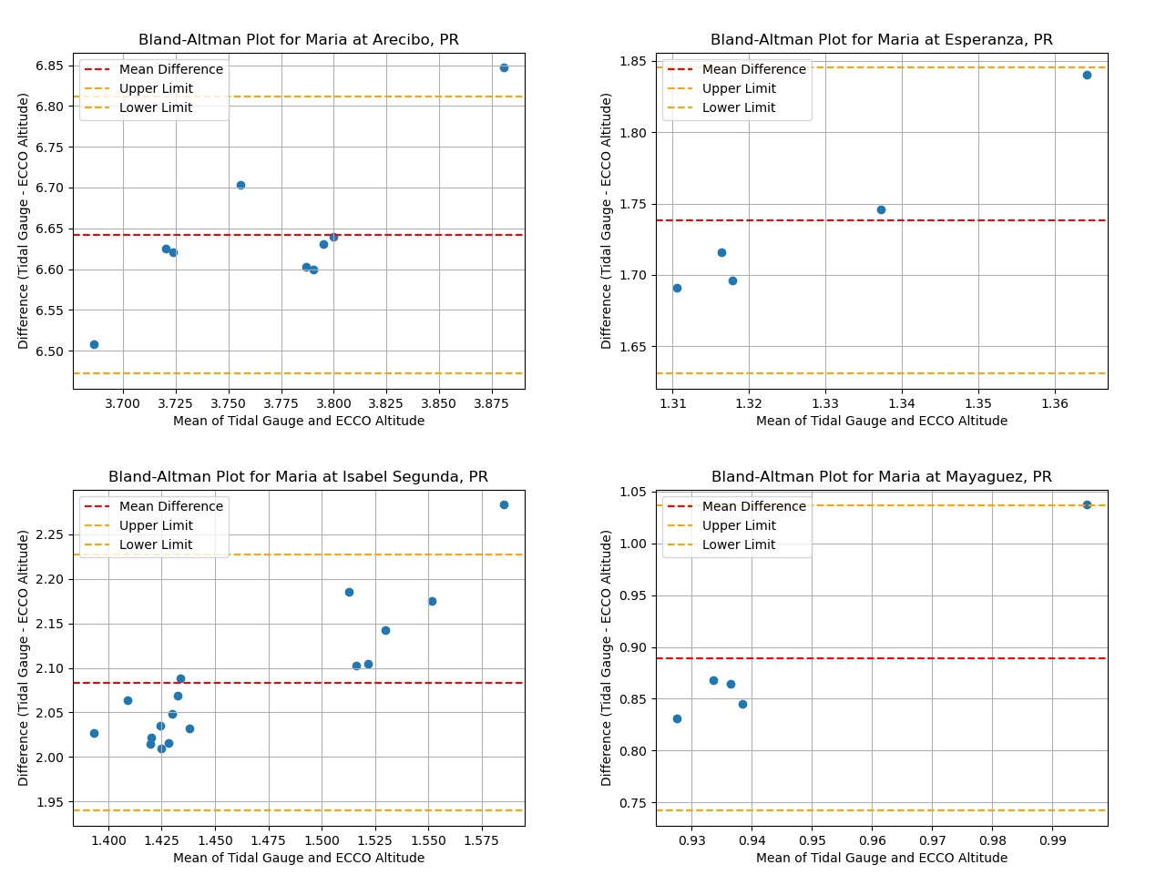
We use Bland–Altman plots to determine the correlation between the SSH data from ECCO and UHSLC. A Bland–Altman plot, also known as a difference plot, is a plot comparing two measurement techniques and assessing the agreement between two sets of data. It provides a visual representation of the difference between two measurements on the y-axis and the average of the two measurements on the x-axis [8]. However, before generating Bland-Altman plots, we determine if it is possible to plot for all locations by running the following code:
for event in ar_allLoc_allEvent_tg.keys():
        for locat in ar_allLoc_allEvent_tg[event].keys():
            try: plot_bland_altman(event, locat, ar_allLoc_allEvent_tg, ar_allLoc_allEvent_sat, save_fig=True, plot_fig=False)
            except: print(f"Excluded:\tevent: {event}\t\tLocation: {locat}")
Output:
Excluded: event: Maria Location: Fajardo, PR
From the output, we see that SSH data from Fajardo cannot be plotted using Bland-Altman, hence it is excluded.
To generate the Bland-Altman plots, we define the following function:
def plot_bland_altman(event, locat, ar_allLoc_allEvent_tg, ar_allLoc_allEvent_sat):
    tidal_gauge = ar_allLoc_allEvent_tg[event][locat]
    satellite_altimetry = ar_allLoc_allEvent_sat[event][locat]

    differences = tidal_gauge - satellite_altimetry

    if len(differences) == 0 or np.all(np.isnan(differences)):
        fig, ax = plt.subplots()
        ax.text(0.5, 0.5, 'No data', fontsize=12, ha='center', va='center')
        ax.axis('off')
        plt.title(f'No Data for {event} at {locat}')
    else:
        mean_difference = np.nanmean(differences)
        std_difference = np.nanstd(differences)
        upper_limit = mean_difference + 1.96 * std_difference
        lower_limit = mean_difference - 1.96 * std_difference

        plt.scatter(np.mean([tidal_gauge, satellite_altimetry], axis=0), differences)
        plt.axhline(mean_difference, color='red', linestyle='--', label='Mean Difference')
        plt.axhline(upper_limit, color='orange', linestyle='--', label='Upper Limit')
        plt.axhline(lower_limit, color='orange', linestyle='--', label='Lower Limit')
        plt.xlabel('Mean of Tidal Gauge and ECCO Altitude')
        plt.ylabel('Difference (Tidal Gauge - ECCO Altitude)')
        plt.title(f'Bland-Altman Plot for {event} at {locat}')
        plt.legend()
        plt.grid(True)

        plt.show()
To generate a Bland-Altman plot for Arecibo, for example, we call the function like this:
plot_bland_altman("Maria", "Arecibo, PR", ar_allLoc_allEvent_tg, ar_allLoc_allEvent_sat)
The following Bland-Altman plots are generated for Arecibo, Esperanza, Isabel Segunda and Mayaguez:
Plotting
We then call the functions described earlier to generate the required plots.
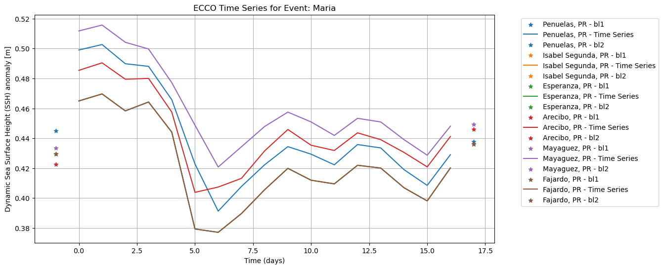
To plot the ECCO SSH data:
plot_time_series(
    ar_allLoc_allEvent_sat,
    baseline_dict = bl_allLoc_allEvent_sat,
    event = "Maria",
    type = "ECCO",
    xlabel = "Time (days)",
    ylabel = "Dynamic Sea Surface Height (SSH) anomaly [m]",
    save_fig=True,
    plot_fig=True
    )
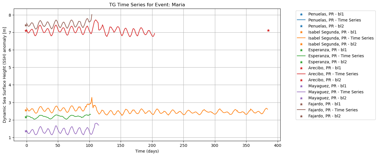
To plot the UHSLC SSH data:
plot_time_series(
    ar_allLoc_allEvent_tg,
    baseline_dict = bl_allLoc_allEvent_tg,
    event = "Maria",
    type = "TG",
    xlabel = "Time (days)",
    ylabel = "Dynamic Sea Surface Height (SSH) anomaly [m]",
    save_fig=True,
    plot_fig=True
    )
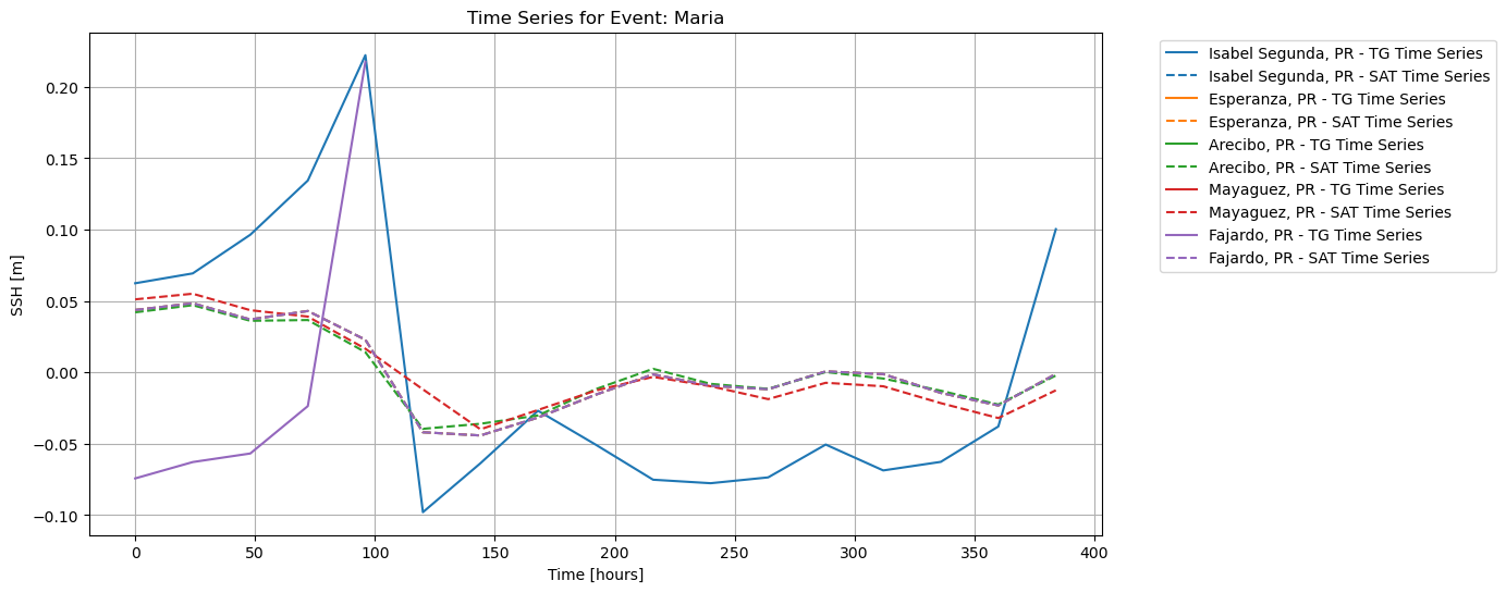
To plot both ECCO and UHSLC SSH, normalized and resampled:
plot_time_series_combined(
    ar_allLoc_allEvent_tg,
    ar_allLoc_allEvent_sat,
    event = "Maria",
    xlab="Time [hours]", ylab="SSH [m]",
    baseline_dict=True,
    normalize_zero=True,
    resample_tg=True,
    save_fig=True, plot_fig=True)
To plot both ECCO and UHSLC SSH normalized, but not resampled:
plot_time_series_combined(
    ar_allLoc_allEvent_tg,
    ar_allLoc_allEvent_sat,
    event = "Maria",
    xlab="Time [hours]", ylab="SSH [m]",
    baseline_dict=True,
    normalize_zero=True,
    resample_tg=False,
    save_fig=True, plot_fig=True)
Discussion
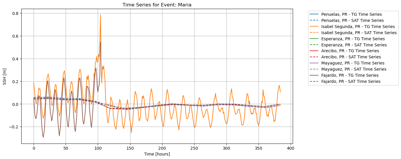
From our analysis, the data visualizations resampled to similar time steps appear to show a linear relationship between the ECCO and UHSLC SSH data, since the UHSLC SSH data increases over the same time steps with the ECCO SSH data in the same location. However, the correlation values do not agree, showing a lack of correlation of ECCO SSH data during extreme storm events. Moreover, in the Bland-Altman analyses, we see that the disagreement between ECCO and UHSLC SSH data increases with increasing sea surface height, showing that extreme weather events contribute to greater differences in the measured values of sea level between data systems.
Furthermore, there are benefits and disadvantages of each of our SSH data sources. Tide gauges offer unmatched temporal resolution, and they are very useful in detecting small changes in sea level rise due to tides, given their in situ location. However, they are highly suspectible to damage during extreme storm events, which renders them useless. Unlike tide gauges, satellite sources, for example ECCO, are not affected by extreme weather events, but they cannot capture changes during short time scales when tides occur.
We decided to extend our analysis to the entire SSH dataset, to see if our findings from the preliminary analysis still hold for SSH data unaffected by extreme weather events, such as storms.
SSH data analysis of the entire dataset
We perform some analyses on the data and generate plots to observe any trends in the SSH data obtained from ECCO and UHSLC. For both data sources, we find, compare and plot the following:
- rolling mean comparison
- rolling standard deviation comparison
- pearson correlation of the rolling mean and rolling standard deviation
- pearson correlation for the entire time series
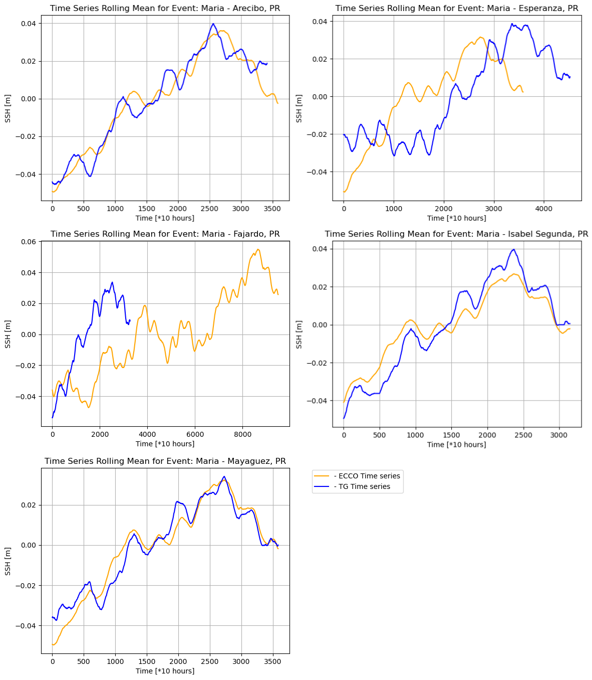
To compress and smoothen the temporal coarseness of the SSH data, both ECCO and UHSLC time series data were put through a 1000-hour rolling window to compute the mean and standard deviation. Then we find the pearson correlation coefficient and p-value by comparing the rolling mean and rolling standard deviation obtained from both the ECCO and UHSLC SSH data. The Pearson coefficient is a mathematical correlation coefficient representing the relationship between two variables [9].
Rolling mean comparison
ds_allLoc_allEvent_ec and ds_allLoc_allEvent_tg are dictionaries in which the SSH datasets from ECCO and UHSLC have been saved respectively. To access the ECCO data for Hurricane Maria in Arecibo, we can call ds_allLoc_allEvent_ec["Maria"]["Arecibo, PR"]. We then convert the SSH data from millimeters into meters by dividing by 1000. After that, the data is normalized and plotted.
ds_m_avg_sat = ds_allLoc_allEvent_ec[event_to_process][loc_to_process].SSH.rolling(time=1000, min_periods=1, center=True).mean()
ds_m_avg_tg = ds_allLoc_allEvent_tg[event_to_process][loc_to_process].sea_level.rolling(time=1000, min_periods=1, center=True).mean()
ds_m_avg_tg = ds_m_avg_tg / 1000

ds_m_avg_sat_normalized = ds_m_avg_sat - ds_m_avg_sat.mean()
ds_m_avg_tg_normalized = ds_m_avg_tg - ds_m_avg_tg.mean()

plt.plot(ds_m_avg_sat_normalized, color='orange', label=f' - ECCO Time series')
plt.plot(ds_m_avg_tg_normalized.values.flatten(), color='blue', label=f' - TG Time series')

plt.xlabel("Time [*10 hours]")
plt.ylabel("SSH [m]")
plt.title(f"Time Series Rolling Mean for Event: {event_to_process} - {loc_to_process}")
plt.legend(bbox_to_anchor=(1.05, 1.0), loc='upper left')
plt.grid(True)
plt.show()
The following plots are generated for all the locations:
Rolling standard deviation comparison
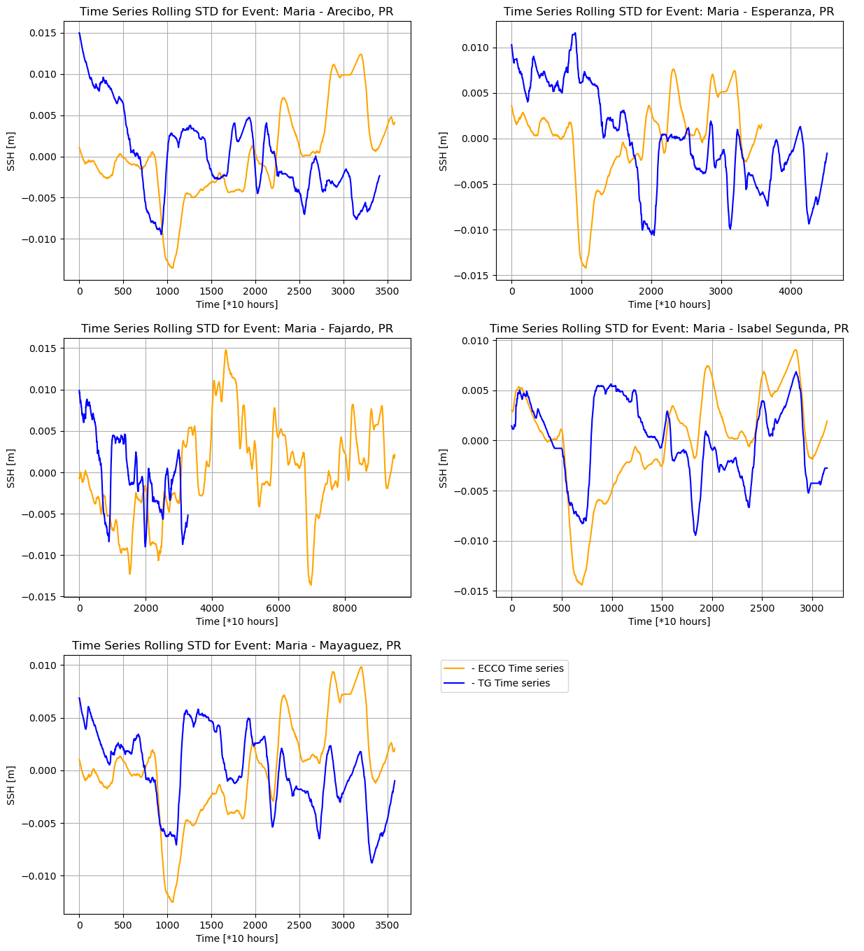
The same code can be reused to generate plots for the rolling standard deviation comparison by making a few changes to the variables to be plotted, as shown below.
-ds_m_avg_sat_normalized = ds_m_avg_sat - ds_m_avg_sat.mean()
-ds_m_avg_tg_normalized = ds_m_avg_tg - ds_m_avg_tg.mean()
+ds_m_std_sat_normalized = ds_m_std_sat - ds_m_std_sat.mean()
+ds_m_std_tg_normalized = ds_m_std_tg - ds_m_std_tg.mean()
The following plots are then generated for all the locations:
Pearson correlations
We also compute the pearson correlation coefficient and p-value comparing the SSH data from ECCO and UHSLC for each location. We create a function make_arrays_same_length, which ensures that both data arrays in the comparison are of the same length.
def make_arrays_same_length(arr1, arr2):
    len1, len2 = len(arr1), len(arr2)

    if len1 != len2:
        min_len = min(len1, len2)
        arr1 = arr1[:min_len]
        arr2 = arr2[:min_len]

    return arr1, arr2
We can calculate the pearson correlation and p-value of the standard deviation for Isabel Segunda as shown below, using SciPy’s pearsonr() function [10].
corr_val_ds_ec = ds_m_std_sat_normalized
corr_val_ds_tg = ds_m_std_tg_normalized.values.flatten()

corr_val_ds_ec, corr_val_ds_tg = make_arrays_same_length(corr_val_ds_ec, corr_val_ds_tg)

correlation_coefficient, p_value = pearsonr(corr_val_ds_ec, corr_val_ds_tg)

print(f"Pearson correlation coefficient: {correlation_coefficient}")
print(f"P-value: {p_value}")
Output:
Pearson correlation coefficient: 0.3865297618168296
P-value: 9.630575093800546e-113
Time series plotting
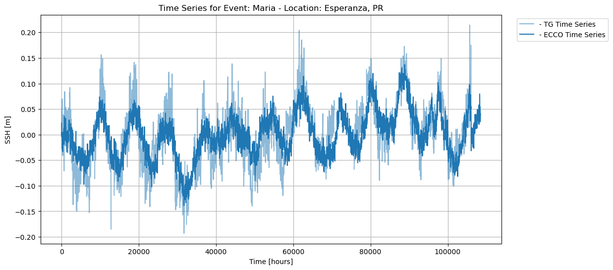
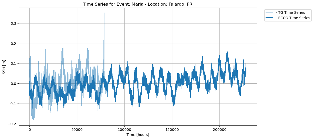
Finally, we plot the time series for the entire dataset for both ECCO and UHSLC SSH data, for each tidal gauge location, to see the overall comparison of the SSH data sources, during and outside of extreme weather events.
plot_time_series_specific_location(
    ar_allLoc_allEvent_tg,
    ar_allLoc_allEvent_ec,
    event_to_process,
    location= 'Isabel Segunda, PR',
    xlab="Time [hours]", ylab="SSH [m]",
    normalize_zero=True,
    resample_tg=True,
    save_fig=True, plot_fig=True)
Time series plot of SSH data from ECCO and UHSLC during Hurricane Maria:
Discussion
Pearson coefficients show correlation, and range from +1 to -1, with +1 representing a positive correlation, -1 representing a negative correlation, and 0 representing no relationship [9]. The pearson’s correlation coefficients and p-values for the rolling mean and rolling standard deviation are shown in the table below:

We can observe the following relationships: Fajardo, Mayaguez, and Arecibo show a strong positive correlation, Esperanza shows a moderate positive correlation and Isabel Segunda shows a weak positive correlation for the rolling mean, while Isabel Segunda shows a weak positive correlation, Esperanza and Arecibo show a weak negative correlation, and Mayaguez and Fajardo show almost no correlation for the rolling standard deviation. We also observe very low standard deviation values, depicting low variations in the respective data sources. However, there is a somewhat low correlation in the rolling standard deviation between the ECCO and UHSLC SSH data.
In addition, the time series analysis showing the intersection between ECCO and UHSLC SSH data reveals that the data is incomplete for some time series, i.e., Fajardo, suggesting that the tide gauge was destroyed due to extreme weather.
Overall, we make similar conclusions to the preliminary analysis. ECCO is fairly reliable over long time scales, however, it does not account for rise in sea level due to extreme weather events. Furthermore, although tide gauges seem more accurate over short time scales, especially in depicting rise in sea level during extreme events, they are vulnerable to extreme weather. Thus in situ sources can be unreliable during extreme events since tide gauges can be destroyed.
Conclusion
Notes
- The code for this project can be found here.
- If you would like to watch the presentation of our project during the Climatematch Impact Scholar Program (CISP) seminar, you can find the video recording here.
- You can also find the slides for the preliminary analysis presentation here and the CISP program presentation here.
Acknowledgements
Most of this work was developed during the Climatematch Impact Scholars Program hosted by Climatematch Academy. Computing and storage resources during the program were supported by ‘An Open, Community Supported, Accessible Summer School for Climate Science, National Aeronautics and Space Administration’ (Award #80NSSC23K0835). I would like to thank my teammates, Franck and Hannah, who I worked with in this project, and Fabrizio Falasca, who mentored us during the latter part of the project.
References
[1] Sea Level Rise - Woods Hole Oceanographic Institution: https://www.whoi.edu/know-your-ocean/ocean-topics/climate-weather/sea-level-rise/
[2] What is a tide gauge?: https://oceanservice.noaa.gov/facts/tide-gauge.html
[3] Ichikawa, K., Wang, X., Tamura, H., & Wei, D. (2022). Sea surface height and significant wave height estimations in the calm semienclosed Celebes Sea. Coastal Altimetry, 109-134. https://doi.org/10.1016/B978-0-323-91708-7.00011-0
[4] Sea Level Trends - NOAA Tides and Currents: https://tidesandcurrents.noaa.gov/sltrends/
[5] ECCO Version 4 Release 4 Dataset ECCO Consortium, Fukumori, I., Wang, O., Fenty, I., Forget, G., Heimbach, P., & Ponte, R. M. ECCO Central Estimate (Version 4 Release 4). Retrieved from https://data.nas.nasa.gov/ecco/data.php?dir=/eccodata/llc_90/ECCOv4/Release4
[6] ECCO Consortium, Fukumori, I., Wang, O., Fenty, I., Forget, G., Heimbach, P., & Ponte, R. M. (2021, February 10). Synopsis of the ECCO Central Production Global Ocean and Sea-Ice State Estimate (Version 4 Release 4). https://doi.org/10.5281/zenodo.4533349
[7] Forget, G., J.-M. Campin, P. Heimbach, C. N. Hill, R. M. Ponte, and C. Wunsch, 2015: ECCO version 4: An integrated framework for non-linear inverse modeling and global ocean state estimation. Geoscientific Model Development, 8. https://www.geosci-model-dev.net/8/3071/2015/
[8] Bland-Altman plot(simply explained) - DATAtab: https://datatab.net/tutorial/bland-altman-plot
[9] What Is the Pearson Coefficient? Definition, Benefits, and History: https://www.investopedia.com/terms/p/pearsoncoefficient.asp
[10] scipy.stats.pearsonr - SciPy v1.13.1 Manual: https://docs.scipy.org/doc/scipy/reference/generated/scipy.stats.pearsonr.html